Home » Articles

Evaluation Metrics in Machine Learning

In this article, we will learn about the evaluation metrics, evaluation metrics for regression, evaluation metrics for classification. By IncludeHelp Last updated : April 03, 2023

Pursuing a machine learning job is a solid choice for a high-paying career that will be in demand for decades. They have jumped by almost 75 percent over the past four years and will keep growing. There’s a place for you regardless of the specialty you choose to pursue. More importantly, machine learning is poised to impact every industry, and your field may eventually need such experts. And the best investment to make inorder to become an industry expert is to join a professional course.

As we know, Loss functions and evaluation metrics are frequently mixed up. A machine learning model's training process uses a loss function to measure how far the expected and actual outputs diverge. An estimate of the model's performance on the training data is provided by a loss function. In most cases, loss functions can be differentiated based on the model's parameters. Because a gradient descent optimization technique updates the parameters based on the loss value to help the model become more predictive.

On the other hand, evaluation metrics are used to assess the performance of the model after it has been trained and need to be differentiable. However, certain loss functions also serve as evaluation metrics. Typically, we find these kinds of loss functions in regression problems. For example, the below-discussed MSE and MAE act as both loss functions and evaluation metrics.

In this article, we will discuss the performance metrics for both regression and classification tasks.

Evaluation Metrics for Regression

• Mean Squared Error (MSE)
• Mean Absolute Error (MAE)
• R² Coefficient of Determination

Mean Squared Error (MSE)

Mean Squared Error (MSE) is a widely used statistical measure used in regression analysis to evaluate the quality of the model's predictions. MSE is defined as the average of the squared differences between the original and the predicted values.

Mathematically, MSE is calculated by subtracting the predicted value from the actual value, squaring the result, and then averaging the squared differences over the entire dataset.

The formula for MSE is:

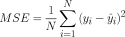
yi = dependent variable's actual value for observation I, I = forecast value, and N = total no.of observations.

Properties of MSE

• MSE is differentiable, so it can be easily implemented.
• MSE is sensitive to outliers, as the squared differences are magnified for larger errors. This can cause the model to be overly influenced by outliers.
• MSE assumes that the errors are normally distributed with a mean of zero, which may not always be the case in practice.
• It can be challenging to interpret the absolute value of MSE, as it depends on the scale of the dependent variable.

Mean Absolute Error (MAE)

Similar to MSE, MAE is a metric that quantifies the discrepancy between the predicted and actual values. However, unlike MSE, MAE computes the absolute value of the differences between predicted and actual values instead of squaring them.

Mathematically, MAE is calculated by subtracting the predicted value from the actual value, taking the absolute value of the result, and then averaging the absolute differences over the entire dataset.

The formula for MAE is:

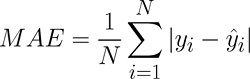
where N = no.of observations, I = predicted value of the dependent variable for observation I and yi = dependent variable's actual value for observation i.

Properties of MAE

• MAE is robust to outliers compared to MSE, as it does not magnify the effect of large errors.
• It is easier to interpret the absolute value of MAE as it is on the same scale as the dependent variable.
• Like MSE, MAE assumes that the errors are normally distributed with a mean of zero, which may not always be the case in practice.
• MAE is differentiable except at x=0, whereas MSE is differentiable at all values of x.

R² Coefficient of Determination

The R² (pronounced "R-squared") coefficient of determination is another statistical measure used to evaluate the performance of regression models.

R² represents the proportion of the variance in the dependent variable (target) that is explained by the independent variables in the model (regression line).

Generally, the value of R² lies between 0 and 1. Higher the R² value, the better the fit. The calculation of R² involves determining the ratio of the variance that is explained by the model to the total variance:

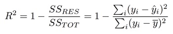
Where, SS_RES is the sum of squares of the residuals (i.e., the differences between the actual and predicted values), and SS_TOT is the total sum of squares (i.e., the sum of squares of the differences between the actual values and the mean value of the dependent variable).

Properties of R²

• R² is independent of the scale of the dependent variable, which makes it useful for comparing models that use different units of measurement.
• R² is less sensitive to the scale of the dependent variable than MSE and MAE.
• R² does not tell you anything about the magnitude of the errors.

Evaluation Metrics for Classification

• Confusion Matrix (Not a measure)
• Accuracy
• Precision
• Recall
• F1-score
• AU-ROC

Confusion Matrix

The confusion matrix is a visual representation in a table format that compares the predicted labels by a model with the actual labels. It is not a loss function or evaluation metric by itself. However, it can be used to calculate various evaluation metrics like precision, recall, accuracy, F1-score, etc.

These metrics give insights into the model's performance on a specific dataset. The rows in the confusion matrix correspond to the predicted class instances, while the columns represent the actual class instances. It is a matrix of four values that summarize the no. of correct and incorrect predictions made by the model.

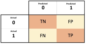
Here,

• True +ve (TP) refers to the count of accurate predictions where the model correctly identifies a +ve class.
• False +ve (FP) indicates the no.of inaccurate predictions where the model incorrectly identifies a +ve class.
• True Negative (TN) represents the count of accurate predictions where the model correctly identifies a negative class.
• False Negative (FN) is a term used to describe the quantity of incorrect predictions in which the model erroneously assigns a negative class.

Accuracy

Accuracy is a performance metric that measures how successfully a predictive model can classify or forecast the intended variable. It is frequently employed in statistics and machine learning. Accuracy = dividing the total no.of predictions by the no.that the model accurately anticipated.

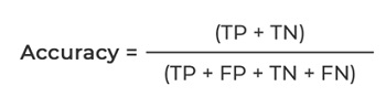
The formula for accuracy is:

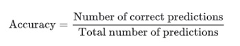
In terms of the type of predictions made by the model, accuracy can be defined as:

Properties of Accuracy

• Easy to understand: Accuracy is a simple and intuitive metric that can be easily interpreted by non-technical stakeholders, such as business managers and executives.
• Provides a general overview: Accuracy provides a general overview of how well a classification model is performing, making it useful for high-level analysis and decision-making.
• Useful for balanced datasets: Accuracy is a useful metric when the dataset is balanced, meaning that the no. of +ve and negative samples is roughly equal. In such cases, accuracy can be a good indicator of model performance.
• Biased towards majority class: Accuracy can be biased towards the majority class in imbalanced datasets, where the no. of +ve and negative samples is significantly different. In such cases, a model can achieve high accuracy by simply predicting the majority class, even if it performs poorly on the minority class.
• Ignores the cost of misclassification: Accuracy treats all misclassifications equally, regardless of their consequences. In some scenarios, misclassifying a +ve sample as negative can be more costly than misclassifying a negative sample as +ve.

Precision

A classification model's precision is the percentage of true +ve predictions among all +ve predictions. It is derived by dividing the total of true +ves (TP) and false +ves by the no.of true +ves (TP) (FP).

The formula for precision is:

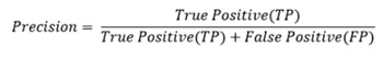
Precision provides information about the quality of the +ve predictions made by a model. A high precision score means that a model is making few false +ve predictions, which means that it is correctly identifying the +ve class with a high degree of confidence. In contrast, a low precision score means that a model is making many false +ve predictions, which means that it is incorrectly identifying the negative class as +ve.

Precision is often used in scenarios where the cost of a false +ve prediction is high, such as in a medical diagnosis, where a false +ve result can lead to unnecessary medical procedures or treatments. In such cases, a high precision score is desirable, as it means that the model is making fewer false +ve predictions, reducing the risk of unnecessary procedures.

For a complete performance, it should be used in conjunction with other evaluation measures like recall and F1-score.

Recall

In a classification model, recall quantifies the percentage of true +ve predictions made among all real +ve samples. It is computed by dividing the total of true +ves (TP) and false negatives (FN) by the no.of true +ves (TP) (FN).

The formula for the recall is:

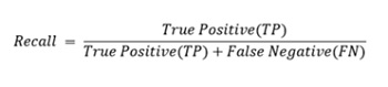
Recall provides information about the completeness of the +ve predictions made by a model. A high recall score means that a model is correctly identifying a high proportion of the +ve class, indicating that it is sensitive to +ve samples. In contrast, a low recall score means that a model is missing many +ve samples, indicating that it is not sensitive to +ve samples.

Recall is often used in scenarios where the cost of a false negative prediction is high, such as in a medical diagnosis, where a false negative result can lead to a delayed diagnosis or treatment. In such cases, a high recall score is desirable, as it means that the model is correctly identifying more +ve samples, reducing the risk of missed diagnoses.

It's worth mentioning that recall should not be used as a sole metric for evaluation as it doesn't consider false +ve predictions, which occur when a negative sample is inaccurately identified as +ve. Hence, it is advisable to utilize it in combination with other evaluation metrics like Precision and F1-score to gain a comprehensive understanding of the model's performance.

F1-score

The F1-score is a single value that combines recall and precision. It is calculated as follows and represents the harmonic mean of recall and precision:

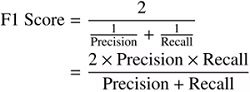
Since both false +ves and false negatives are essential, the F1-score offers a balanced measure of precision and recall, making it valuable. A model with a high F1-score has high precision and recall, properly identifying the +ve class with the least amount of erroneous +ve and false negative predictions.

F1-score is especially useful in scenarios where the dataset is imbalanced, as it takes into account both false +ve and false negative predictions. In such cases, a model that simply predicts the majority class may have high accuracy but may have low precision and recall on the minority class, resulting in a low F1-score.

It is crucial to remember that the F1-score, which gives equal weight to precision and recall, may not always be the optimal statistic to utilize. Other metrics, such as precision or recall, may be more relevant in some situations, such as medical diagnosis, where the cost of a false +ve or false negative prediction may differ.

AU-ROC

Area Underneath the Operational Receiver AU-ROC is the name of the characteristic curve. This is a typical assessment metric used to gauge the efficiency of binary classification models in machine learning. At different categorization thresholds, the true +ve rate (TPR), also known as sensitivity, is shown against the false +ve rate (FPR), also known as 1-specificity.

AU-ROC has several advantages as an evaluation metric. It is insensitive to class imbalance, making it a useful metric for imbalanced datasets. It also provides a good measure of the discrimination ability of a model and allows for easy comparison of different models.

AU-ROC is constrained in some ways, though. The expenses related to false +ves and false negatives are not considered. The cost of a false +ve or false -ve prediction may change in some situations, such as medical diagnosis, and other measures, such as precision or recall, may be more applicable. A model's performance in particular parts of the ROC curve may not be adequately reflected by AU-ROC since it can be affected by the dataset's distribution.

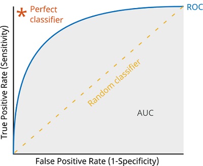
Image source

Advanced Learning

For advanced learning,

Reader can explore Huber Loss, Logarithmic loss, Adjusted R², F-beta score, Why harmonic mean is used in F1-score instead of arithmetic mean, Confusion matrix for multi-class classification, Macro F1-score, Micro F1 score, mean Average Precision (mAP), NDCG (Normalized Discounted Cumulative Gain).