Home » Data Science

Simple Linear Regression in Data Science

Data Science | Simple Linear Regression: In this tutorial, we are going to learn about the Simple Linear Regression in Data Science, Alright, Formula, etc.
Submitted by Kartiki Malik, on March 24, 2020

Simple Linear Regression

A simple regression model could be a linear approximation of a causative relationship between two or additional variables. Regressions models are extremely valuable, as they're one in every of the foremost common ways that to create inferences and predictions.

The process goes like this. You get sample data, come back up with a model that explains the data and so create predictions for the total population supported the model you've developed.

There is a variable, labeled Y, being foreseen, and freelance variables, tagged x1, x2, so forth. These are the predictors. Y could be a perform of the X variables, and also the regression model could be a linear approximation of this perform.

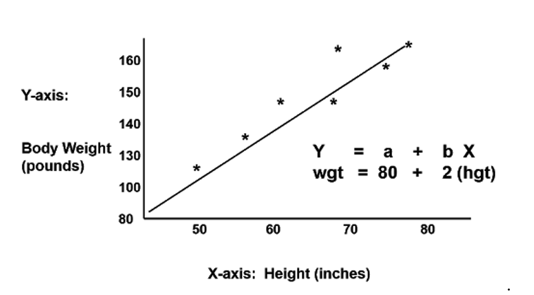
The easiest regression model is that the straightforward linear regression: Y is up to beta zero and beta one-time x plus epsilon.

Let's see what these values mean. Y is that the variable we tend to are attempting to predict and is termed the variable. X is a variable quantity. Once exploitation multivariate analysis, we wish to predict the worth of Y, provided we have the worth of X.

But to possess a regression, Y should depend upon X in some causative manner. Whenever there's a modification in X, such modification should translate into a change in Y.

Think about the subsequent equation: the financial gain an individual receives depends on the number of years of education that a person has received. The variable is financial gain, whereas the variable quantity is years of education. There's a causative relationship between the 2. The additional education you get, the upper the financial gain you're possible to receive. This relationship is therefore trivial that it's in all probability the explanation you're observing this course, right now. You would like to urge better financial gain, therefore you're increasing your education.

Now, let's pause for a second and have faith in the reverse relationship. What if education depends on financial gain. This might mean the upper your financial gain, the additional years you pay educating yourself. Golf shot high tuition fees aside, wealthier people don't pay additional years in class. And, highschool and faculty take a similar range of years, regardless of your income bracket. Therefore, a causative relationship like this one is faulty, if not plain wrong. Hence, it's unfit for multivariate analysis.

Let's return to the initial example. Financial gain could be a performance of education. The additional years you study, the upper financial gain you'll receive. This sounds regarding right.

Alright

What we haven't mentioned, so far, is that, in our model, there are coefficients. Beta one is the constant that stands before the variable quantity. It quantifies the result of education on financial gain. If beta one is fifty, then for every further year of education, your financial gain would grow by $50. In the USA, the amount is way larger, somewhere around three to 5,000 bucks. So, for every further year you pay on education, your yearly financial gain is predicted to rise by 3 to 5 thousand bucks. And that's not considering pedagogy or tailored courses, like this one.

The different 2 other parts are the constant beta zero and also the error – epsilon.
In this example, you'll be able to consider the constant beta zero because of the pay. Regardless of your education, if you have got employment, you'll get the pay. This is often a secured quantity.

So, if you have never visited the college and plug an education worth of zero years within the formula, the regression can predict that your financial gain is going to be the pay smart, right?

The last term is epsilon. This represents the error of estimation. The error is that the actual distinction between the determined financial gain and also the income the regression foreseen. On average, across all observations, the error is zero. If you earn over what the regression has foreseen, then somebody earns but what the regression has foreseen. Everything evens out.

Formula

The original formula was written with Greek letters. What will this tell us? it was the population formula. However, we all know statistics are all regarding sample information. In follow, we tend to use the statistical regression equation.

It is merely y hat equals b zero plus b one time x.

You detected right. The y here is noted as y hat. Whenever we have a hat image, it's calculable or a foreseen worth.

b zero is that the estimate of the regression constant beta zero, whereas b one is that the estimate of beta one, and x is that the sample information for the variable quantity.