Home »
Data Analytics
Data Analytics – Probability, Its Distribution, and Types
Learn what is probability, what is probability distribution, types of probability distribution, etc.
Submitted by IncludeHelp, on April 06, 2022
What is Probability?
Probability is a mathematical term that expresses the probability of anything happening and forecasts the likelihood of certain events occurring.
What is Probability Distribution?
A probability distribution is a statistical function. For a random variable within a range, a probability distribution describes all the possible values and probabilities. It is also defined as a set of possible outcomes of any random experiment. These settings can be a set of real numbers, vectors, or entities.
Types of Probability Distribution
The probability distribution is divided into two parts:
- Discrete Probability Distributions
- Continuous Probability Distributions
1. Discrete Probability Distribution
A discrete distribution expresses the probability of occurrence of each value of a discrete random variable. Discrete variables create a discrete probability distribution. If a random variable is discrete, the probability distribution will be discrete. These distributions are used to describe the probability of random variables with discrete outcomes.
For example,
Example 1: the set 0, 1, 2 indicates the potential values for the random variable X, which reflects the number of heads that can occur when a coin is tossed twice.
Example 2: A dice is rolled. You earn a gift if you roll a six.
Example 3: Estimate the man's weight. You can win a reward if your prediction is within ten pounds.
In a discrete probability distribution, each potential value of the discrete random variable can be linked with a non-zero probability.
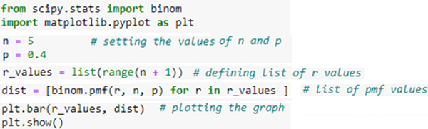
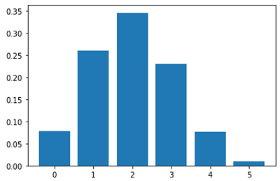
Binomial Distribution
In statistics, the binomial distribution is one of the most widely used distributions. It estimates the probability of achieving k successes in n binomial experiments. Hence, a discrete distribution with a finite number of possibilities is the binomial distribution. The binomial distribution develops from a sequence of what are known as Bernoulli trials. A Bernoulli trial is a scientific test that has only two possible outcomes: success or failure.
Consider a six-time toss of a biassed coin with a 0.4 probability of landing on the head. If a "success" is defined as "getting a head," the binomial distribution will provide the probability of r successes for each value of r.
The number of successes (r) in n consecutive independent Bernoulli trials is represented by the binomial random variable.
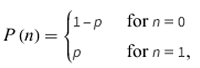
Bernoulli's Distribution
The Bernoulli distribution is a form of the Binomial distribution in which just one experiment is carried out, yielding only one observation. As a result, the Bernoulli distribution is used to explain occurrences with possible outcomes. Mathematically this is described as –
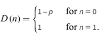
The Bernoulli distribution is a discrete distribution having two possible outcomes labeled by n=0 and n=1, here n=1 denotes”success” occurs with probability p and n=0 denotes”failure" occurs with probability q=1-p, where 0<p<1. It therefore has probability density function.
This can be written as –
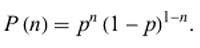
The corresponding distribution function is
Here's the implementation of Bernoulli distribution using Python has described below:
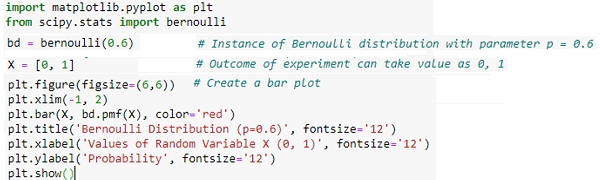
The anticipated value of a Bernoulli random variable is p, which is also known as the Bernoulli distribution's parameter. Bernoulli random variables have two possible values: 0 and 1. The result of the experiment might be a value of 0 or 1. The probability of various random variable values is calculated using the pmf function.
Poisson Distribution
In statistics, a Poisson distribution is a probability distribution that shows how many times an event is expected to occur over a certain period of time. Therefore; the Poisson distribution is a discrete distribution that assesses the probability of a certain number of events occurring in a particular time period. When we know how often something happens, a Poisson distribution can help us to anticipate the probability of its happening again. It tells us the chances of a certain number of occurrences occurring in a certain amount of time.
Poisson distribution is a count distribution, to put it another way. Poisson distributions are widely used to understand independent events that occur at a steady rate across time. The name was inspired by Siméon Denis Poisson, a French mathematician.
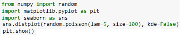
A basic example of Poisson distribution is shown in the Python code below.
There are two parameters to it:
- Lam: Number of instances known
- Size: The returned array's size.
The 1x100 distribution for occurrence 5 is generated using the Python method below.
2. Continuous Probability Distributions
A continuous distribution describes the probabilities of a continuous random variable's possible values. A continuous random variable has an infinite and uncountable set of possible values (known as the range). The mapping of time can be considered as an example of the continuous probability distribution. It can be from 1 second to 1 billion seconds, and so on.
The area under the curve of a continuous random variable's PDF is used to calculate its probability. As a result, only value ranges can have a non-zero probability. A continuous random variable's probability of equaling some value is always zero.
Followings are the types of the continuous probability distribution.
Normal Distribution
One of the most fundamental continuous distribution types is the normal distribution. It's also known as a Gaussian distribution. This probability distribution is symmetrical around its mean value. There is a centre to the probability distribution of a normal distribution, which is centered on the mean. This indicates that the distribution has more data around the mean than the mean itself. As we move away from the centre, the distribution of data becomes less even. The resulting curve is symmetrical about the mean and has the shape of a bell-shaped probability distribution. Consider the following graph, which depicts the probability distribution of heights within a certain class of individuals:
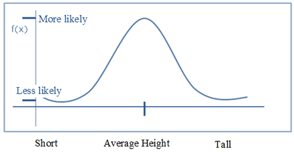
Figure: Illustration of the Normal Distribution
As we can see from the graph above, the distribution is centred on the mean, which is the average of all heights in the population. Aside from this, the majority of the data is in the vicinity of the mean. As we go away from the location, the probability density reduces as well. This type of curve is referred to as a Bell Curve, and it is a characteristic of a normal distribution that is common. It also shows that data that is near to the mean is more common than data that is distant from it. The variance is a finite value, and the mean is 0.
Continuous Uniform Distribution
It is possible to have an unlimited number of measurable values with a continuous number of equally likely measurable values when using a continuous uniform distribution also known as a rectangle distribution. In contrast to discrete random variables, a continuous random variable can take on any real value within a specified range, unlike discrete random variables.
All outcomes are equally feasible in a continuous uniform distribution. As a consequence, each variable has the same probability of getting it. In this symmetric probabilistic distribution, random variables are spread equally with a 1/ (b-a) probability.
In most cases, a continuous uniform distribution looks like rectangular shape. A random number generator may be considered as a continuous uniform distribution with a constant mean and variance. Every variable has an equal probability of occurring in a continuous uniform distribution, just as it does in a discrete uniform distribution. However, there is no limit to the number of points that can exist at any given time.
Log-Normal Distribution
The log-normal distribution is a continuous probability distribution with a right skewed tail, which means it has a lengthy tail to the right of the distribution's centre. This distribution is used to visualize random variables whose logarithm values follow a normal distribution. Take a look at the X and Y random variables. Y = ln(X), where ln signifies the natural logarithm of X values, is the variable represented in this distribution.
In addition, it is used to model a variety of natural phenomena, such as income distributions, the length of chess games, and the time required to repair a maintainable system, among other things.
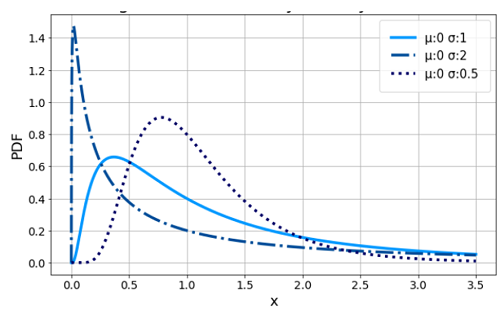
Figure: The probability density curve with a logarithmic scale.
Where x > 0 and the probability density function is specified by the two parameters and, the log-normal probability density function is defined as -
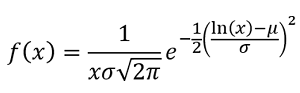
The location parameter of the distribution is denoted by μ, and the scale parameter is denoted by σ. These two quantities should not be confused with the more commonly known mean and standard deviation from a normal distribution, which are the same thing. The mean and standard deviation of our log-normal data can be calculated using logarithms when our log-normal data is transformed using logarithms.
Advertisement
Advertisement