Home » Computer Science Organization

Vector processing, its characteristics and instruction fields | Computer Science Organization

In this article, we will learn about the concept of vector processing, its characteristics and its instruction fields.
Submitted by Shivangi Jain, on August 02, 2018

Vector processing

The need to increase computational power is a never-ending requirement. In scientific and research areas, the computational involved are quite extensive and hence high power computers are the must.

The areas like structural engineering, petroleum exploration, aerodynamics, hydrodynamics, nuclear research, tomography, VLSI design, AI can have data in the form of matrices which suits vector processors to process it at a high speed.

Some examples of its are:

1. In radar and signal processing for detection of space / underwater targets.
2. In remote sensing for earth resources exploration.
3. In computational wind tunnel experiments.
4. In 3D stop-action computer assisted tomography.
5. Weather forecasting.
6. Medical diagnosis.

Characteristics of Vector processing

1. A vector is an ordered set of elements. A vector operand contains an ordered set of n elements, where n is called the length of the vector. Each element in a vector is a scalar quantity, which may be floating point number, an integer, a logical value, or a character (byte).
2. In vector processing, two successive pairs of elements are processed each clock period. In dual vector pipes and dual sets of vector functional units allow two pairs of elements to be processed during the same clock period. As each pair of operations is completed, the results are delivered to the appropriate elements of the result register. The operation continues until the number of elements processed is equal to the count specified by the vector length register.
   For example: C (1:50) = A (1:50) + B (1:50)
   This vector instruction includes the initial addresses of the two source operands, one destination operand, the length of the vectors and the operation to be performed.
3. Vector instructions are classified into for basic types:

       F1: V = V	f2: V = S
       F3: V * V = V 	f4: V*S = V

Where V indicates vector operand and S indicates scalar operand. The operations f1 and f2 are unary operations such as vector square root, vector sine, vector complement, vector summation and so on. On the other hand, operations f3 and f4 are binary operations such as vector add, vector multiply, vector scalar adds and so on.
4. In vector processing, identical processes are repeatedly invoked many times, each of which can be subdivided into subprocesses.
5. In vector processing, successive operands are fed through the pipeline segments and require as few buffers and local controls as possible. This parallel vector processing allows the generation of more than two results per clock period. The parallel vector operations are automatically initiated either when successive vector instructions use different functional units and different vector registers, or when successive vector instructions use the result stream from one vector register as the operand of another operation using different functional units. This process is known as chaining.
6. Because of the startup delay in a pipeline, a vector processor performs better with longer vectors.
7. Vector processing is usually faster and more efficient than scalar processing because it reduces the overhead associated with maintenance of the loop control variables.

Vector Instruction Fields

Vector instructions are usually specified by the following fields:

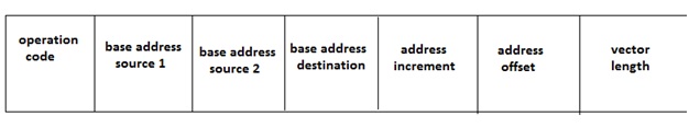
1. Opcode (operation code):
   This field is used to select the functional unit or to reconfigure a multifunctional unit to perform the specified operation.
2. Base addresses:
   In case of memory reference instruction, this field specifies the base addresses needed for source operands and result vectors. If the operands and results are located in the vector register file, the designated vector registers must be specified.
3. Address increment:
   This field specifies the space between the two elements in the main memory. Usually, the elements are consecutively stored thus the increment is 1. However, with variable increment higher flexibility can be offered in the applications.
4. Address offset:
   This field specifies the offset to the base address. Using the base address and the offset, the effective memory address can be calculated. The offset can be either positive or negative.
5. Vector length:
   this field determines the termination of a vector instruction. Vector length affects the processing efficiency because the additional subdividing is required for long vectors.