Home » Machine Learning/Artificial Intelligence

Pearson Coefficient of Correlation in Machine Learning

In this tutorial, we will learn about the Pearson coefficient of correlation in machine learning, and its implementation using Python. By Raunak Goswami Last updated : April 16, 2023

Pearson's Correlation

Pearson's correlation helps us to understand the relationships between the feature values (independent values) and the target value (dependent value or the value to be predicted ) which will further help us in improving our model’s efficiency.

How to Calculate Pearson's Correlation?

Mathematically pearson's correlation is calculated as:

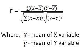
So now the question arises, what should be stored in the variable X and what should be stored in variable Y. We generally store the feature values in X and target value in the Y. The formula written above will tell us whether there exists any correlation between the selected feature value and the target value.

Before we code there are few basic things that we should keep in mind about correlation:

• The value of Correlation will always lie between 1 and -1
• Correlation=0, it means there is absolutely no relationship between the selected feature value and the target value.
• Correlation=1, it means that there is a perfect relationship between the selected feature value and the target value and this would mean that the selected feature is appropriate for our model to learn.
• Correlation=-1, it means that there exists a negative relationship between the selected feature value and the target value, generally, the use of the feature value having a negative value of low magnitude is discouraged for e.g. -0.1 0r -0.2.

Python Code to Implement Pearson Correlation

The data set used can be downloaded from here: headbrain3.CSV

"""
# -*- coding: utf-8 -*-
"""
Created on Sun Jul 29 22:21:12 2018
@author: Raunak Goswami
"""
import numpy as np
import pandas as pd
import matplotlib.pyplot as plt
"""

#reading the data
"""
here the directory of my code and the headbrain3.csv file 
is same make sure both the files are stored in same folder
or directory
""" 
data=pd.read_csv('headbrain3.csv')

#this will show the first five records of the whole data
data.head()

w=data.iloc[:,0:1].values
y=data.iloc[:,1:2].values
#this will create a variable x which has the feature values i.e head size
x=data.iloc[:,2:3].values
#this will create a variable y which has the target value i.e brain weight
z=data.iloc[:,3:4].values 

print(round(data['Gender'].corr(data['Brain Weight(grams)'])))          
plt.scatter(w,z,c='red')
plt.title('scattered graph for coorelation between Gender and brainweight' )
plt.xlabel('age')
plt.ylabel('brain weight')
plt.show()

print(round(data['Age Range'].corr(data['Brain Weight(grams)'])))          
plt.scatter(x,z,c='red')
plt.title('scattered graph for coorelation between age and brainweight' )
plt.xlabel('age range')
plt.ylabel('brain weight')
plt.show()

print(round((data['Head Size(cm^3)'].corr(data['Brain Weight(grams)']))))         
plt.scatter(x,z,c='red')
plt.title('scattered graph for coorelation between head size and brainweight' )
plt.xlabel('head size')
plt.ylabel('brain weight')
plt.show()

data.info()
data['Head Size(cm^3)'].corr(data['Brain Weight(grams)'])
k=data.corr()
print("The table for all possible values of pearson's coefficients is as follows")
print(k)

After you run your code in Spyder tool provided by anaconda distribution just go to your variable explorer and search for the variable named as k and double-click to see the values in that variable and you’ll see something like this

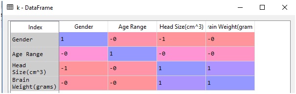
The table above shows the correlation values here 1 means perfect correlation,0 is for no correlation and -1 stands for negative correlation.

Now let us understand these values using the graphs:

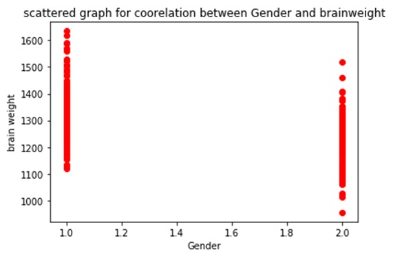
The reason for getting this abruptly looking graph is that there is no correlation between gender and brain weight, that is why we cannot use gender as a feature value in our prediction model.Let us try drawing graph for brain weight using another feature value, what about head size?

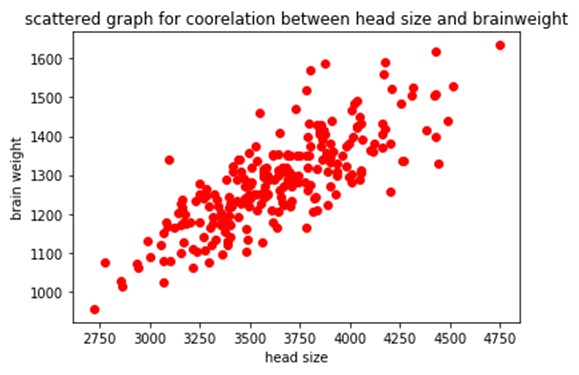
As you can see in the table, there exists a perfect correlation between between brain weight and head size so as a result we a getting a definite graph this signifies that there exists a perfect linear relationship between brain weight and head size so we can use head size as one of the feature value in our model.

That is all for this article if you have any queries just write in the comment section I would be happy to help you. Have a great day ahead, keep learning.

---