Home » Machine Learning/Artificial Intelligence

Spearman's Correlation and Its Implementation using Python

In this tutorial, we will learn about the Spearman's correlation and Its implementation using Python. By Raunak Goswami Last updated : April 16, 2023

Overview

This article is about correlation and its implementation in the machine learning. In my previous article, I have discussed Pearson's correlation coefficient and later we have written a code to show the usefulness of finding Pearson's correlation coefficient.

Difference Between Pearson's and Spearman's Correlation

Pearson's correlation works fine only with the linear relationships whereas Spearman's correlation works well even with the non-linear relationships.

Another advantage of using Spearman's correlation is that since it uses ranks to find the correlation values, therefore, this correlation well suited for continuous as well as discrete datasets.

Formula of Spearman's Correlation

The Spearman's rank correlation coefficient is:

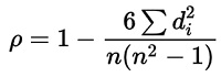
Where,

• d_i: The difference between the two ranks of each observation
• n: The number of observations

Here, the the value of dican be calculated as X-Y where X= feature values and Y= target values.

Spearman's Correlation Implementation using Python

The Dataset used can be downloaded from here: headbrain4.CSV

Since we have used the continuous dataset. i.e. the same dataset used for Pearson's correlation, you will not be able to observe much of a difference between the Pearson and Spearman correlation, you can download any discrete dataset and you'll see the difference.

So now, let us see how we can use Spearman's correlation in our machine learning program using python programming:

# -*- coding: utf-8 -*-
"""
Created on Sun Jul 29 22:21:12 2018

@author: Raunak Goswami
"""

import numpy as np
import pandas as pd
import matplotlib.pyplot as plt

#reading the data
"""
here the directory of my code and the headbrain4.csv 
file is same make sure both the files are stored in 
the same folder or directory
""" 
data=pd.read_csv('headbrain4.csv')

#this will show the first five records of the whole data
data.head()

#this will create a variable w which has the feature values i.e Gender
w=data.iloc[:,0:1].values
#this will create a variable x which has the feature values i.e Age Range
y=data.iloc[:,1:2].values
#this will create a variable x which has the feature values i.e head size
x=data.iloc[:,2:3].values
#this will create a variable y which has the target value i.e brain weight
z=data.iloc[:,3:4].values 



print(round(data['Gender'].corr(data['Brain Weight(grams)'],method='spearman')))          
plt.scatter(w,z,c='red')
plt.title('scattered graph for Spearman correlation between Gender and brainweight' )
plt.xlabel('Gender')
plt.ylabel('brain weight')
plt.show()


print(round(data['Age Range'].corr(data['Brain Weight(grams)'],method='spearman')))          
plt.scatter(x,z,c='red')
plt.title('scattered graph for Spearman correlation between age and brainweight' )
plt.xlabel('age range')
plt.ylabel('brain weight')
plt.show()



print(round((data['Head Size(cm^3)'].corr(data['Brain Weight(grams)'],method='spearman'))))         
plt.scatter(x,z,c='red')
plt.title('scattered graph for Spearman correlation between head size and brainweight' )
plt.xlabel('head size')
plt.ylabel('brain weight')
plt.show()

data.info()
data['Head Size(cm^3)'].corr(data['Brain Weight(grams)'])
k1=data.corr(method='spearman')
print("The table for all possible values of spearman's coeffecients is as follows")
print(k1)

After you run your code in Spyder tool provided by anaconda distribution just go to your variable explorer and search for the variable named as k1 and double-click to see the values in that variable and you'll see something like this:

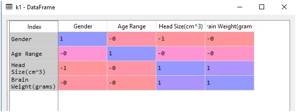
Here,1 signifies a perfect correlation,0 is for no correlation and -1 signifies a negative correlation.

As you look carefully, you will see that the value of the correlation between brain weight and head size is always 1. If you remember were getting a similar value of correlation in Pearson's correlation

Now, just go to the ipython console you will see some self-explanatory scattered graphs, in case you are having any trouble understanding those graphs just have a look at my previous article about Pearson's correlation and its implication in machine learning and you'll get to know.

---